38 how to change excel chart data labels to custom values
How to hide zero data labels in chart in Excel? - ExtendOffice If you want to hide zero data labels in chart, please do as follow: 1. Right click at one of the data labels, and select Format Data Labels from the context menu. See screenshot: 2. In the Format Data Labels dialog, Click Number in left pane, then select Custom from the Category list box, and type #"" into the Format Code text box, and click Add button to add it to Type list box. excel - How do I update the data label of a chart? - Stack Overflow Select the data label Then, place your cursor in Excel's Formula Bar, and enter the formula like ='Sheet2'!$C$3. Now, that data label is associated by the formula, to the cell C3, which contains the desired data label that we built above. Repeat as needed. Note: The sheet name is required in this formula.
Make your Excel charts easier to read with custom data labels the Data Labels tab and, in the Label Contains section, click the Value check box. Click Next. Click Finish. Right-click one of the data markers in the chart. Select Format Data...

How to change excel chart data labels to custom values
Excel Custom Chart Labels • My Online Training Hub Step 1: Select cells A26:D38 and insert a column Chart. Step 2: Select the Max series and plot it on the Secondary Axis: double click the Max series > Format Data Series > Secondary Axis: Step 3: Insert labels on the Max series: right-click series > Add Data Labels: Step 4: Change the horizontal category axis for the Max series: right-click ... How to add and customize chart data labels - Get Digital Help Edit data labels. Excel allows you to edit the data label value manually, simply press with left mouse button on a data label until it is selected. Press with left mouse button on again to select the text, you can now type any value you want. I changed the data label value to "Look here!". You can link a group of data labels to a cell range so ... Add or remove data labels in a chart - Microsoft Support Add data labels to a chart · Click the data series or chart. · In the upper right corner, next to the chart, click Add Chart Element · To change the location, ...
How to change excel chart data labels to custom values. Data Labels in Excel Pivot Chart (Detailed Analysis) Click on the Plus sign right next to the Chart, then from the Data labels, click on the More Options. After that, in the Format Data Labels, click on the Value From Cells. And click on the Select Range. In the next step, select the range of cells B5:B11. Click OK after this. Custom Data Labels with Colors and Symbols in Excel Charts - [How To ... To apply custom format on data labels inside charts via custom number formatting, the data labels must be based on values. You have several options like series name, value from cells, category name. But it has to be values otherwise colors won't appear. Symbols issue is quite beyond me. Add or remove data labels in a chart When the Data Label Range dialog box appears, go back to the spreadsheet and select the range for which you want the cell values to display as data labels. When you do that, the selected range will appear in the Data Label Range dialog box. Then click OK. The cell values will now display as data labels in your chart. Custom Excel Chart Label Positions • My Online Training Hub Custom Excel Chart Label Positions - Setup. The source data table has an extra column for the 'Label' which calculates the maximum of the Actual and Target: The formatting of the Label series is set to 'No fill' and 'No line' making it invisible in the chart, hence the name 'ghost series': The Label Series uses the 'Value ...
Is there a way to change the order of Data Labels? Answer Rena Yu MSFT Microsoft Agent | Moderator Replied on April 4, 2018 Report abuse Hi Keith, I got your meaning. Please try to double click the the part of the label value, and choose the one you want to show to change the order. Thanks, Rena ----------------------- * Beware of scammers posting fake support numbers here. Create Dynamic Chart Data Labels with Slicers - Excel Campus Step 6: Setup the Pivot Table and Slicer. The final step is to make the data labels interactive. We do this with a pivot table and slicer. The source data for the pivot table is the Table on the left side in the image below. This table contains the three options for the different data labels. Edit titles or data labels in a chart - support.microsoft.com The first click selects the data labels for the whole data series, and the second click selects the individual data label. Right-click the data label, and then click Format Data Label or Format Data Labels. Click Label Options if it's not selected, and then select the Reset Label Text check box. Top of Page How to create Custom Data Labels in Excel Charts - Efficiency 365 Two ways to do it. Click on the Plus sign next to the chart and choose the Data Labels option. We do NOT want the data to be shown. To customize it, click on the arrow next to Data Labels and choose More Options … Unselect the Value option and select the Value from Cells option. Choose the third column (without the heading) as the range.
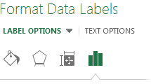
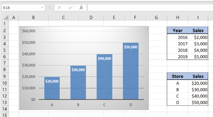
How to Use Cell Values for Excel Chart Labels - How-To Geek Select the chart, choose the "Chart Elements" option, click the "Data Labels" arrow, and then "More Options." Uncheck the "Value" box and check the "Value From Cells" box. Select cells C2:C6 to use for the data label range and then click the "OK" button. The values from these cells are now used for the chart data labels. How to Change Excel Chart Data Labels to Custom Values? - Chandoo.org May 05, 2010 · First add data labels to the chart (Layout Ribbon > Data Labels) Define the new data label values in a bunch of cells, like this: Now, click on any data label. This will select “all” data labels. Now click once again. At this point excel will select only one data label. Go to Formula bar, press = and point to the cell where the data label for that chart data point is defined. How to Customize Your Excel Pivot Chart Data Labels - dummies If you want to label data markers with a category name, select the Category Name check box. To label the data markers with the underlying value, select the Value check box. In Excel 2007 and Excel 2010, the Data Labels command appears on the Layout tab. Also, the More Data Labels Options command displays a dialog box rather than a pane. Change the format of data labels in a chart To get there, after adding your data labels, select the data label to format, and then click Chart Elements > Data Labels > More Options. To go to the appropriate area, click one of the four icons ( Fill & Line, Effects, Size & Properties ( Layout & Properties in Outlook or Word), or Label Options) shown here.
Enable or Disable Excel Data Labels at the click of a button ...
Custom Excel Chart Label Positions - YouTube Customize Excel Chart Label Positions with a ghost/dummy series in your chart. Download the Excel file and see step by step written instructions here: https:...

Change Horizontal Axis Values in Excel 2016 - AbsentData
Using the CONCAT function to create custom data labels for an Excel chart Use the chart skittle (the "+" sign to the right of the chart) to select Data Labels and select More Options to display the Data Labels task pane. Check the Value From Cells checkbox and select the cells containing the custom labels, cells C5 to C16 in this example.
Create a Custom Number Format for a Chart Axis
Chart.ApplyDataLabels method (Excel) | Microsoft Learn The type of data label to apply. True to show the legend key next to the point. The default value is False. True if the object automatically generates appropriate text based on content. For the Chart and Series objects, True if the series has leader lines. Pass a Boolean value to enable or disable the series name for the data label.

Excel charts: add title, customize chart axis, legend and ...
Custom data labels in a chart - Get Digital Help Press with mouse on "Add Data Labels". Press with mouse on Add Data Labels". Double press with left mouse button on any data label to expand the "Format Data Series" pane. Enable checkbox "Value from cells". A small dialog box prompts for a cell range containing the values you want to use a s data labels.

Solved: How to show all detailed data labels of pie chart ...
Excel custom number formats | Exceljet Measurements. You can use a custom number format to display numbers with an inches mark (") or a feet mark ('). In the screen below, the number formats used for inches and feet are: 0.00 \' // feet 0.00 \" // inches. These results are simplistic, and can't be combined in a single number format.

Google Workspace Updates: Get more control over chart data ...
Excel charts: add title, customize chart axis, legend and data labels Select the chart and go to the Chart Tools tabs ( Design and Format) on the Excel ribbon. Right-click the chart element you would like to customize, and choose the corresponding item from the context menu. Use the chart customization buttons that appear in the top right corner of your Excel graph when you click on it.

Custom data labels in a chart
How to add data labels from different column in an Excel chart? In the Format Data Labels pane, under Label Options tab, check the Value From Cells option, select the specified column in the popping out dialog, and click the OK button. Now the cell values are added before original data labels in bulk. 4. Go ahead to untick the Y Value option (under the Label Options tab) in the Format Data Labels pane.

Excel charts: add title, customize chart axis, legend and ...
How to use cell values for excel chart labels - How to We want to chart the sales values and use the change values for data labels. Use Cell Values for Chart Data Labels. Select range A1:B6 and click Insert > Insert Column or Bar Chart > Clustered Column. The column chart will appear. We want to add data labels to show the change in value for each product compared to last month. Select the chart ...
Change the format of data labels in a chart
excel - Replace "Value From Cells" in chart data labels using VBA ... I have copied several charts from a workbook to another and I managed to change the data series with vba. Some of the data labels of these charts, get data "From Cells" but this range is still referencing the the first workbook and I need to change it to reference the new sheet in the new workbook.I am being able to get the formula that references the "From Cells".

Google Workspace Updates: New chart text and number ...
Excel Charts: Creating Custom Data Labels - YouTube In this video I'll show you how to add data labels to a chart in Excel and then change the range that the data labels are linked to. This video covers both W...
Help Online - Quick Help - FAQ-133 How do I label the data ...
Custom Chart Data Labels In Excel With Formulas - How To Excel At Excel Follow the steps below to create the custom data labels. Select the chart label you want to change. In the formula-bar hit = (equals), select the cell reference containing your chart label's data. In this case, the first label is in cell E2. Finally, repeat for all your chart laebls.
How to Change Axis Values in Excel | Excelchat
Excel charts: how to move data labels to legend @Matt_Fischer-Daly . You can't do that, but you can show a data table below the chart instead of data labels: Click anywhere on the chart. On the Design tab of the ribbon (under Chart Tools), in the Chart Layouts group, click Add Chart Element > Data Table > With Legend Keys (or No Legend Keys if you prefer)

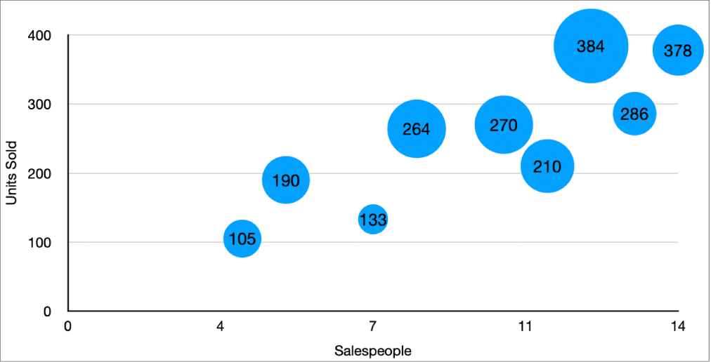
Improve your X Y Scatter Chart with custom data labels
Add or remove data labels in a chart - Microsoft Support Add data labels to a chart · Click the data series or chart. · In the upper right corner, next to the chart, click Add Chart Element · To change the location, ...

Change the format of data labels in a chart
How to add and customize chart data labels - Get Digital Help Edit data labels. Excel allows you to edit the data label value manually, simply press with left mouse button on a data label until it is selected. Press with left mouse button on again to select the text, you can now type any value you want. I changed the data label value to "Look here!". You can link a group of data labels to a cell range so ...

Color Negative Chart Data Labels in Red with downward arrow
Excel Custom Chart Labels • My Online Training Hub Step 1: Select cells A26:D38 and insert a column Chart. Step 2: Select the Max series and plot it on the Secondary Axis: double click the Max series > Format Data Series > Secondary Axis: Step 3: Insert labels on the Max series: right-click series > Add Data Labels: Step 4: Change the horizontal category axis for the Max series: right-click ...

How to Create a Pie Chart in Excel | Smartsheet

Change the format of data labels in a chart

Apply Custom Data Labels to Charted Points - Peltier Tech

Apply Custom Data Labels to Charted Points - Peltier Tech

How to: Display and Format Data Labels | .NET File Format ...

Solved: How to show all detailed data labels of pie chart ...
Directly Labeling Excel Charts - PolicyViz
charts - Excel 2007 - Custom Y-axis values - Super User

how to add data labels into Excel graphs — storytelling with data
Change the look of chart text and labels in Numbers on Mac ...

How to create Custom Data Labels in Excel Charts

Change color of data label placed, using the 'best fit ...

How to Place Labels Directly Through Your Line Graph in ...

Excel charts: add title, customize chart axis, legend and ...

How-to Use Data Labels from a Range in an Excel Chart - Excel ...

How to add data labels from different column in an Excel chart?
How To Create Excel Progress Bar Charts (Professional-Looking!)

Stagger long axis labels and make one label stand out in an ...
Change the look of chart text and labels in Numbers on Mac ...

Change the format of data labels in a chart

Add Labels ON Your Bars

Add or remove data labels in a chart
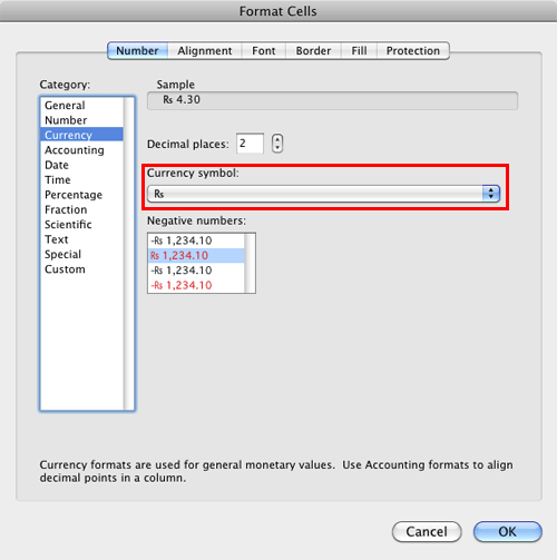
Format Number Options for Chart Data Labels in Excel 2011 for Mac
Post a Comment for "38 how to change excel chart data labels to custom values"