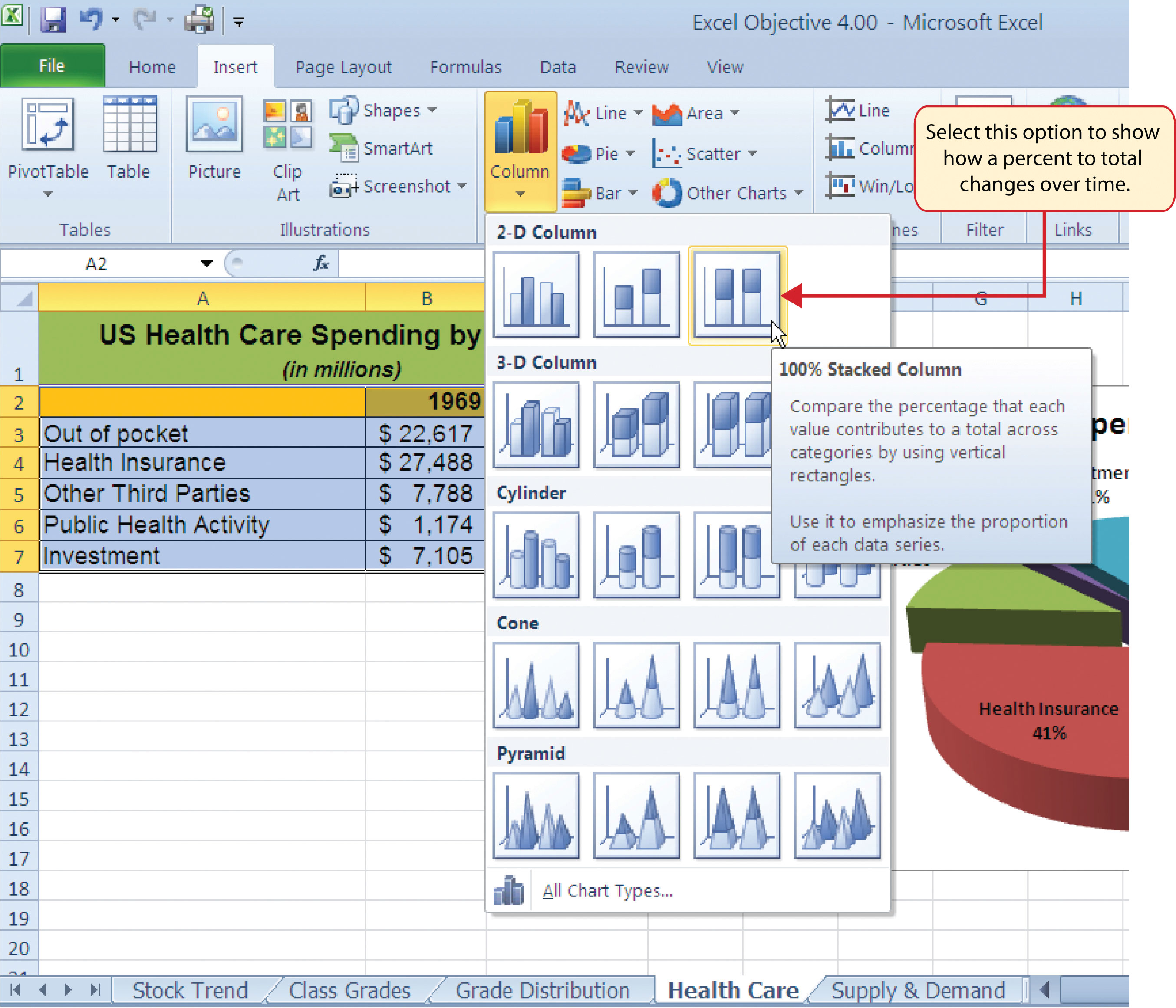
41 use the format data labels task pane to display category name and percentage data labels
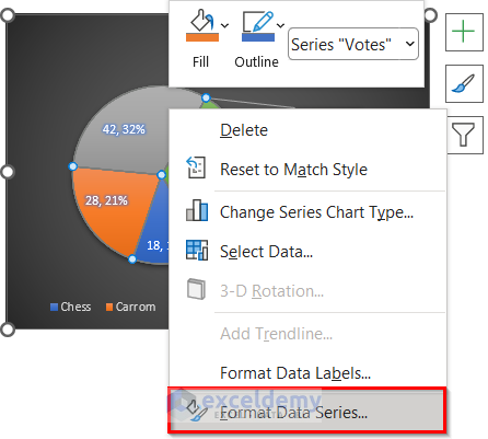
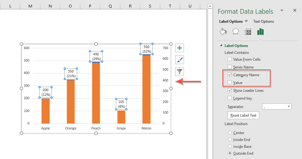
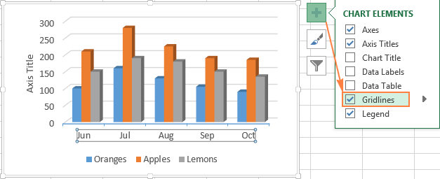
how to display percentage data labels in excel Right click the pie chart again and select Format Data Labels from the right-clicking menu. Select the range I5:I11 and press OK. Uncheck the Value and Show Leader Lines. Most labels have a label content control. However, you can work out this problem with following processes. Change the scale of the horizontal (category) axis in a chart Click anywhere in the chart. This displays the Chart Tools, adding the Design and Format tabs. On the Format tab, in the Current Selection group, click the arrow in the box at the top, and then click Horizontal (Category) Axis. On the Format tab, in the Current Selection group, click Format Selection.
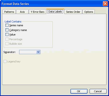
excel 2,3 Flashcards | Quizlet You must make changes to the content of data labels using buttons in the Format Data Labels task pane. true Excel offers two pie chart sub-types, Pie of Pie and Bar of Bar, that can be used to combine many smaller segments of a pie chart into a separate smaller chart.
Use the format data labels task pane to display category name and percentage data labels
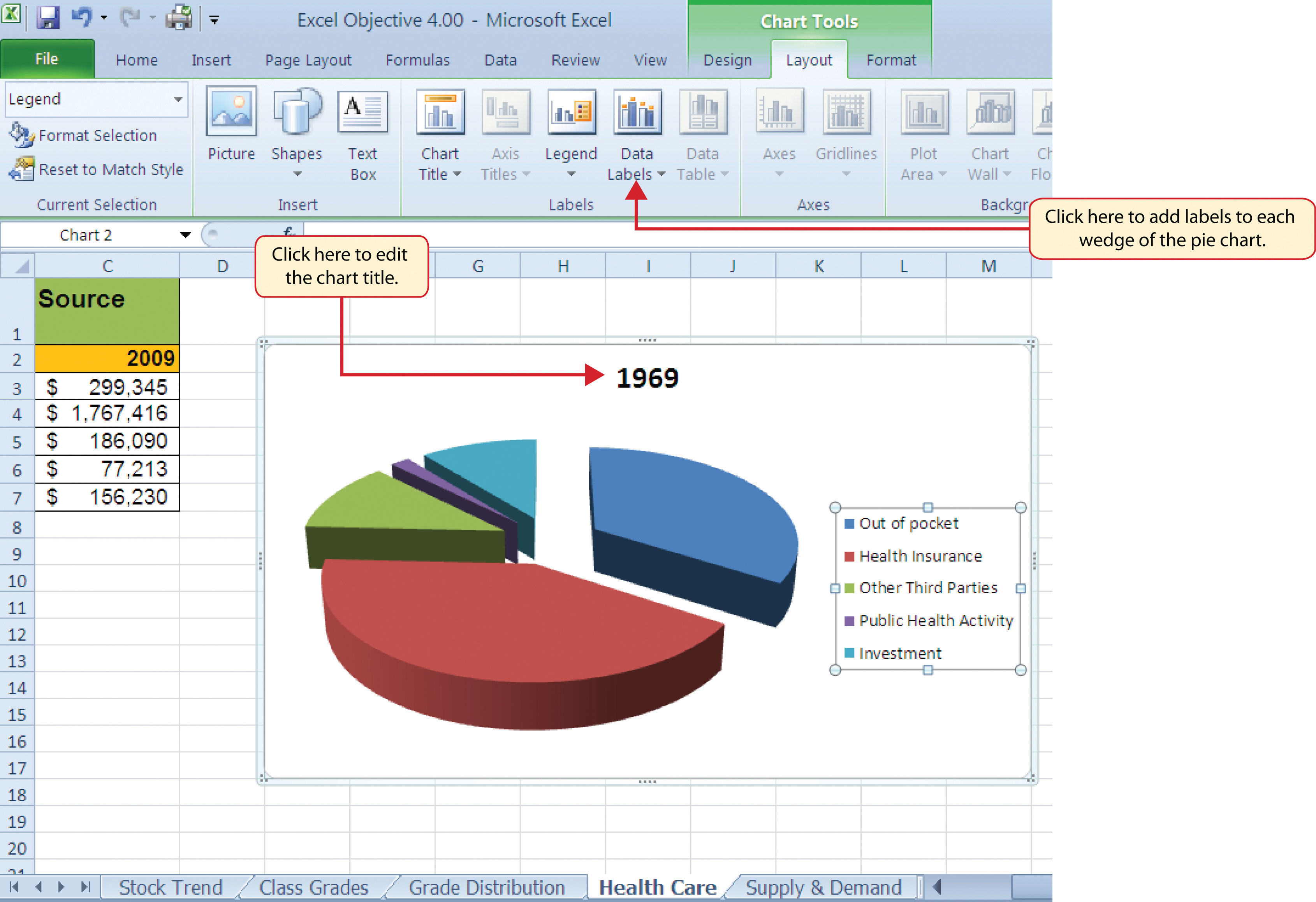
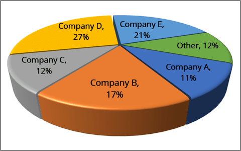
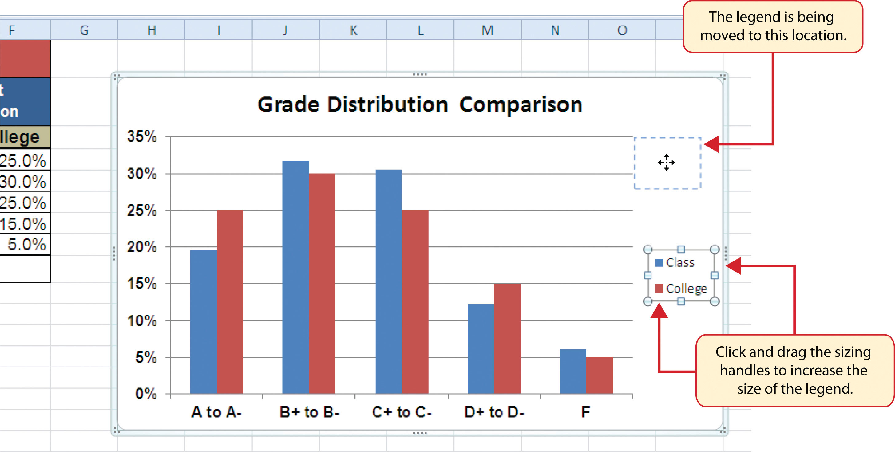
Solved Add Data Callouts as data labels to the 3-D pie - Chegg See the answer. Add Data Callouts as data labels to the 3-D pie chart. Include the category name and percentage in the data labels. Slightly explode the segment of the chart that was allocated the smallest amount of advertising funds. Adjust the rotation of the 3-D Pie chart with a X rotation of 20, a Y rotation of 40, and a Perspective of 10 . Advanced Excel - Quick Guide - tutorialspoint.com The Format pane is a new entry in Excel 2013. It provides advanced formatting options in clean, shiny, new task panes and it is quite handy too. Step 1 − Click on the Chart. Step 2 − Select the chart element (e.g., data series, axes, or titles). Step 3 − Right-click the chart element. Step 4 − Click Format . A data label is descriptive text that shows that - Course Hero Close the Format Data Labels task pane. Click the Home tab and apply font formatting, such as Font Color. To format the legend - Double click the legend to open the Format Legend task pane. Click the Legend Options icon. Select the position of the legend: Top, Bottom, Left, Right, or Top Right. Click the Fill & Line icon, click Border and set border options if you want to change the border settings for the legend. Close the Format Legend task pane. Click the Home tab and apply font ...
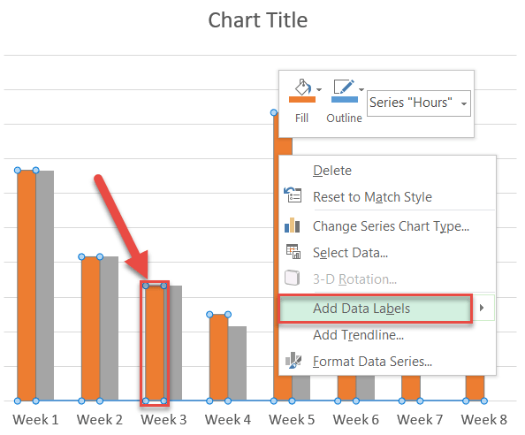
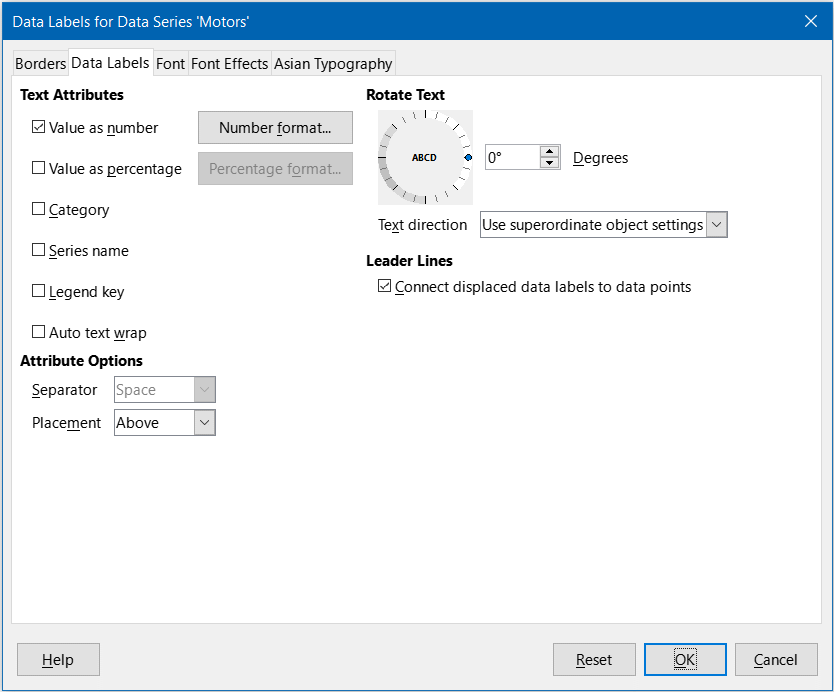
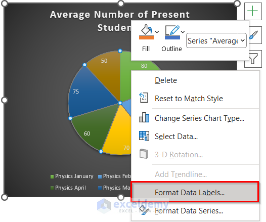
Use the format data labels task pane to display category name and percentage data labels. Excel Chapter 2 - Business Computers 365 Once added, the data labels can be further modified by right-clicking the chart and choosing Format Data Labels to open the Format Data Labels task pane. One or more types of labels can be added and positioned. Adding Category Name labels make the legend redundant. Be careful not to add so many labels that the chart becomes too crowded to read! Format Data Labels in Excel- Instructions - TeachUcomp, Inc. To format data labels in Excel, choose the set of data labels to format. To do this, click the "Format" tab within the "Chart Tools" contextual tab in the Ribbon. Then select the data labels to format from the "Chart Elements" drop-down in the "Current Selection" button group. Formatting Data Labels Select from this drop-down menu of preset formats that can be applied to labels. Custom Format. Select this option to use a custom format. See the following table. Style Labels. Click this button to open the Style dialog box, where you can style text. The Format Labels drop-down menu provides a list of preset formats that you can apply to labels. How to: Display and Format Data Labels - DevExpress In particular, set the DataLabelBase.ShowCategoryName and DataLabelBase.ShowPercent properties to true to display the category name and percentage value in a data label at the same time. To separate these items, assign a new line character to the DataLabelBase.Separator property, so the percentage value will be automatically wrapped to a new line.
Label Options for Chart Data Labels in PowerPoint 2013 for ... - Indezine To do so, first you need to select the Custom option within the Category drop-down list. Then, within the Format Code box, type the required format of the data label numbers to be displayed. Thereafter, click the Add button,highlighted in green within Figure 1, as shown previously on this page, to apply the new format. Change the format of data labels in a chart To get there, after adding your data labels, select the data label to format, and then click Chart Elements > Data Labels > More Options. To go to the appropriate area, click one of the four icons ( Fill & Line, Effects, Size & Properties ( Layout & Properties in Outlook or Word), or Label Options) shown here. Format Data Label Options in PowerPoint 2013 for Windows - Indezine From this menu, choose the Format Data Labels option. Figure 2: Format Data Labels option ; Either of these options opens the Format Data Labels Task Pane, as shown in Figure 3, below. In this Task Pane, you'll find the Label Options and Text Options tabs. These two tabs provide you with all chart data label formatting options. Figure 3: Format Data Labels Task Pane Display the percentage data labels on the active chart. - YouTube Display the percentage data labels on the active chart.Want more? Then download our TEST4U demo from TEST4U provides an innovative approach to learning. Ignore the ...
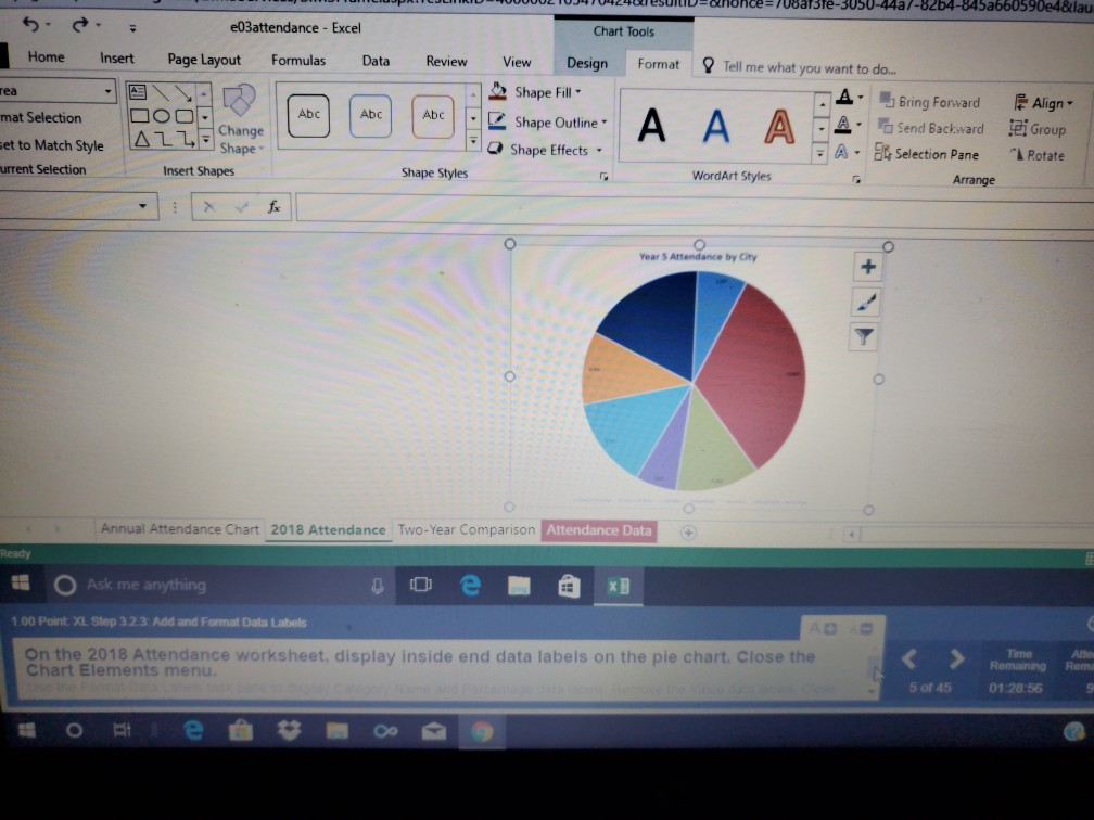
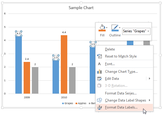
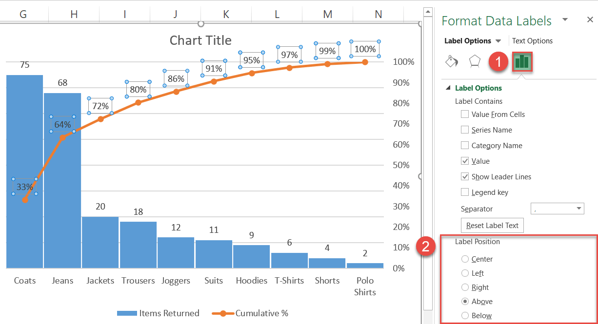
UsetheFormatDataLabelstaskpanetodisplay | Course Hero Use the Format Data Labels task pane to display Percentage data labels and remove the Value data labels. Close the task pane. Apply 18 point size to the data labels. a. Click green plus data labels center click green plus double click in chart label contains click percentage click values check box click close click home font 18 How to Create a Pareto Chart in Excel - Automate Excel To do that, right-click on any of the blue columns representing Series "Items Returned" and click "Format Data Series." Then, follow a few simple steps: Navigate to the Series Options tab. Change "Gap Width" to "3%." Step #7: Add data labels. It's time to add data labels for both the data series (Right-click > Add Data Labels). Creating Pie Chart and Adding/Formatting Data Labels (Excel) Creating Pie Chart and Adding/Formatting Data Labels (Excel) 264,476 views. Jan 20, 2014. 356 Dislike Share Save. Dan Kasper. 1.13K subscribers. Creating Pie Chart and Adding/Formatting Data ... (Get Answer) - Share Format Data Labels Display Outside End data labels ... Share Format Data Labels Display Outside End data labels on the pie chart. Close the Chart Elements menu. Use the Format Data Labels task pane to display Percentage data labels and remove the Value data labels. Close the task pane.
How to Create a Timeline Chart in Excel - Automate Excel
Use grouping and binning in Power BI Desktop - Power BI To use grouping, select two or more elements on a visual by using Ctrl+click to select multiple elements. Then right-click one of the multiple selection elements and choose Group data from the context menu. Once it's created, the group is added to the Legend bucket for the visual. The group also appears in the Fields list.
How to Make a Pie Chart in Excel (5 Suitable Examples)
Custom Number Format in Pie Chart | MrExcel Message Board Sep 2, 2016. #3. - Create a table as shown below. - With Excel 2013 or later, specify the desired range to populate the data labels: format data labels task pane>value from cells>select range. - Important: depending on your regional settings, use commas or dots in the appropriate places at the formula. Charts.
/Capture-e92aa05671d543ceaf94080eb2687619.JPG)
Understanding Excel Chart Data Series, Data Points, and Data ...
Apply Custom Data Labels to Charted Points - Peltier Tech Double click on the label to highlight the text of the label, or just click once to insert the cursor into the existing text. Type the text you want to display in the label, and press the Enter key. Repeat for all of your custom data labels. This could get tedious, and you run the risk of typing the wrong text for the wrong label (I initially ...
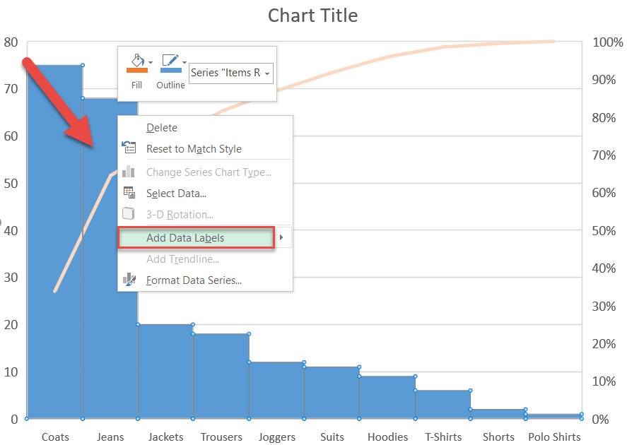
How to Create a Pareto Chart in Excel – Automate Excel
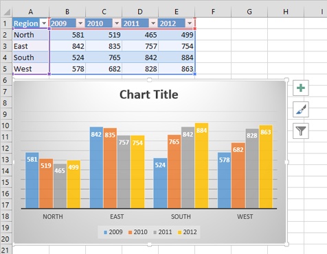
Question : Exp19_Excel_Ch03_ML2_Grades . Steps to Perform: - Chegg Add data labels in the Outside End position for all data series. Format the data series with Blue-Gray, Text 2 fill color. 3. 11. Select the category axis and display the categories in reverse order in the Format Axis task pane so that O'Hair is listed at the top and Sager is listed at the bottom of the bar chart.
Presenting Data with Charts
How to show percentages on three different charts in Excel To convert the calculated decimal values to percentages, right-click on the selected cells and click Format Cells. Alternatively, press CTRL+1 on the keyboard to open the Format Cells dialogue box. 3. In the Format Cells dialogue box, make sure that the Number tab is selected and in the Category list select Percentage.

Creating Pie Chart and Adding/Formatting Data Labels (Excel)
How to show data label in "percentage" instead of - Microsoft Community Select Format Data Labels. Select Number in the left column. Select Percentage in the popup options. In the Format code field set the number of decimal places required and click Add. (Or if the table data in in percentage format then you can select Link to source.) Click OK. Regards, OssieMac. Report abuse.
Chapter 3 Creating Charts and Graphs
cs 385 exam 3 Flashcards | Quizlet Change the data labels from Values to Percentages and then close the Format Data Labels task pane. double click label, select percentage, unselect value, close Sets found in the same folder

Apply Custom Data Labels to Charted Points - Peltier Tech
For formatting your - ipca.passion-lithotherapie.fr In the Chart Elements menu, hover your cursor over the Data Labels option and click on the arrow next to it. 4. In the opened submenu, click on More options. This opens the Format Data Labels task pane. 5. In the Format Data Labels task pane, untick Value and tick the Percentage option to show only percentages.
Question | Chegg.com
A data label is descriptive text that shows that - Course Hero Close the Format Data Labels task pane. Click the Home tab and apply font formatting, such as Font Color. To format the legend - Double click the legend to open the Format Legend task pane. Click the Legend Options icon. Select the position of the legend: Top, Bottom, Left, Right, or Top Right. Click the Fill & Line icon, click Border and set border options if you want to change the border settings for the legend. Close the Format Legend task pane. Click the Home tab and apply font ...
Format Data Label Options in PowerPoint 2013 for Windows
Advanced Excel - Quick Guide - tutorialspoint.com The Format pane is a new entry in Excel 2013. It provides advanced formatting options in clean, shiny, new task panes and it is quite handy too. Step 1 − Click on the Chart. Step 2 − Select the chart element (e.g., data series, axes, or titles). Step 3 − Right-click the chart element. Step 4 − Click Format .
Analyzing Data with Tables and Charts in Microsoft Excel 2013 ...
Solved Add Data Callouts as data labels to the 3-D pie - Chegg See the answer. Add Data Callouts as data labels to the 3-D pie chart. Include the category name and percentage in the data labels. Slightly explode the segment of the chart that was allocated the smallest amount of advertising funds. Adjust the rotation of the 3-D Pie chart with a X rotation of 20, a Y rotation of 40, and a Perspective of 10 .

How to make a pie chart in Excel
Presenting Data with Charts

Analyzing Data with Tables and Charts in Microsoft Excel 2013 ...
Presenting Data with Charts
How to create a chart with both percentage and value in Excel?
How to Create a Pareto Chart in Excel – Automate Excel

Excel charts: add title, customize chart axis, legend and ...

How to make a pie chart in Excel

How to show percentages on three different charts in Excel ...

Formatting Data Labels

Custom data labels in a chart

Change the format of data labels in a chart

How to Use Cell Values for Excel Chart Labels
Excel charts: add title, customize chart axis, legend and ...

Change the format of data labels in a chart

Change the format of data labels in a chart

How to show percentages on three different charts in Excel ...

How to show percentages on three different charts in Excel ...

Display Customized Data Labels on Charts & Graphs
Is it possible to adjust the data label text box dimension in ...

Presenting Data with Charts
How to get an Excel chart to display percentages of each ...
Working with Charts :: Hour 12. Adding a Chart :: Part III ...
Excel 3-D Pie charts - Microsoft Excel 365

Excel Charts - Aesthetic Data Labels

Change the format of data labels in a chart

Excel charts: add title, customize chart axis, legend and ...
Presenting Data with Charts
How to Make a Pie Chart in Excel (5 Suitable Examples)
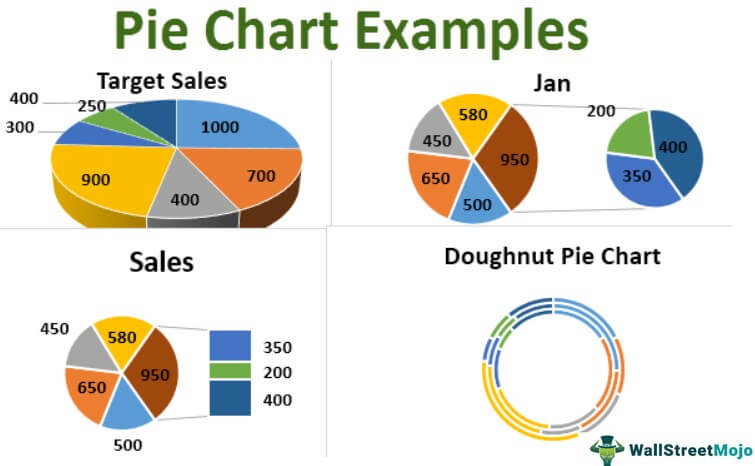
Pie Charts in Excel - How to Make with Step by Step Examples
Post a Comment for "41 use the format data labels task pane to display category name and percentage data labels"