44 data labels excel 2013
January 2022 updates for Microsoft Office Excel 2013. Description of the security update for Excel 2013: January 11, 2022 (KB5002128) Office 2013. Description of the security update for Office 2013: January 11, 2022 (KB5002124) Office 2013. Description of the security update for Office 2013: January 11, 2022 (KB5002064) Office 2013 › excel › how-to-add-total-dataHow to Add Total Data Labels to the Excel Stacked Bar Chart Apr 03, 2013 · Step 4: Right click your new line chart and select “Add Data Labels” Step 5: Right click your new data labels and format them so that their label position is “Above”; also make the labels bold and increase the font size. Step 6: Right click the line, select “Format Data Series”; in the Line Color menu, select “No line”
How to mail merge and print labels from Excel - Ablebits You are now ready to print mailing labels from your Excel spreadsheet. Simply click Print… on the pane (or Finish & Merge > Print documents on the Mailings tab). And then, indicate whether to print all of your mailing labels, the current record or specified ones. Step 8. Save labels for later use (optional)

Data labels excel 2013
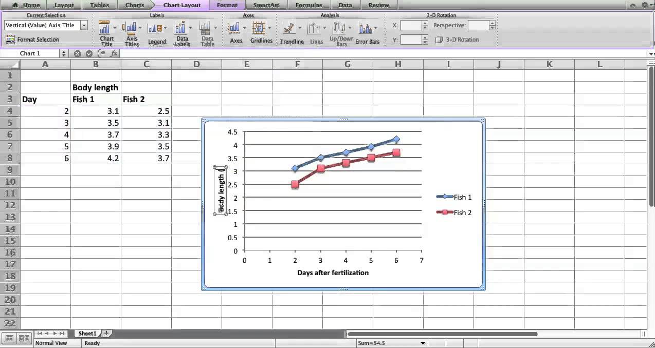
How to Create a Dynamic Chart Title in Excel - Excel Champs Steps to Create Dynamic Chart Title in Excel Converting a normal chart title into a dynamic one is simple. But before that, you need a cell which you can link with the title. Here are the steps: Select chart title in your chart. Go to the formula bar and type =. Select the cell which you want to link with chart title. Hit enter. Excel Waterfall Chart: How to Create One That Doesn't Suck - Zebra BI To create a waterfall chart in Excel 2013 and earlier, you had to define additional data series (with complicated formulas) in the data table and then make them invisible in the chart. And we're not talking about 1 invisible series. If the waterfall chart dipped below zero at one point, you needed at least seven additional series! How to Add Axis Titles in a Microsoft Excel Chart - How-To Geek Select your chart and then head to the Chart Design tab that displays. Click the Add Chart Element drop-down arrow and move your cursor to Axis Titles. In the pop-out menu, select "Primary Horizontal," "Primary Vertical," or both. If you're using Excel on Windows, you can also use the Chart Elements icon on the right of the chart.
Data labels excel 2013. How to Create and Customize a Treemap Chart in Microsoft Excel Select the data for the chart and head to the Insert tab. Click the "Hierarchy" drop-down arrow and select "Treemap." The chart will immediately display in your spreadsheet. And you can see how the rectangles are grouped within their categories along with how the sizes are determined. Using an Excel Table within a data validation list To create the named range, click Formulas -> Define Name The New Name window will open. Give the named range a name ( myDVList in the example below) and set the Refers to box to the name of the Table and column. Finally, Click OK . The named range has now been created. The formula used in the screenshot above is. =myList [Animals] Manage sensitivity labels in Office apps - Microsoft Purview ... Set Use the Sensitivity feature in Office to apply and view sensitivity labels to 0. If you later need to revert this configuration, change the value to 1. You might also need to change this value to 1 if the Sensitivity button isn't displayed on the ribbon as expected. For example, a previous administrator turned this labeling setting off. blogs.library.duke.edu › data › 2012/11/12Adding Colored Regions to Excel Charts - Duke Libraries ... Nov 12, 2012 · Right-click on the individual data series to change the colors, line widths, etc. Use the formatting options or the Chart tools on the Excel ribbon to change the font of any text, adjust the grid lines, add labels and titles, etc. The data series names in the legend can be adjusted by using the “Select Data…” option and typing in custom ...
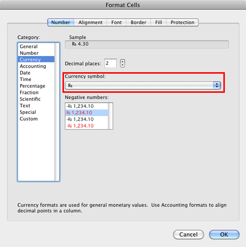
chandoo.org › wp › change-data-labels-in-chartsHow to Change Excel Chart Data Labels to Custom Values? May 05, 2010 · Now, click on any data label. This will select “all” data labels. Now click once again. At this point excel will select only one data label. Go to Formula bar, press = and point to the cell where the data label for that chart data point is defined. Repeat the process for all other data labels, one after another. See the screencast. › make-labels-with-excel-4157653How to Print Labels From Excel - Lifewire Apr 05, 2022 · How to Print Labels From Excel . You can print mailing labels from Excel in a matter of minutes using the mail merge feature in Word. With neat columns and rows, sorting abilities, and data entry features, Excel might be the perfect application for entering and storing information like contact lists. Display data point labels outside a pie chart in a paginated report ... Create a pie chart and display the data labels. Open the Properties pane. On the design surface, click on the pie itself to display the Category properties in the Properties pane. Expand the CustomAttributes node. A list of attributes for the pie chart is displayed. Set the PieLabelStyle property to Outside. Set the PieLineColor property to Black. Custom Excel number format - Ablebits.com To create a custom Excel format, open the workbook in which you want to apply and store your format, and follow these steps: Select a cell for which you want to create custom formatting, and press Ctrl+1 to open the Format Cells dialog. Under Category, select Custom. Type the format code in the Type box. Click OK to save the newly created format.
I do not want to show data in chart that is "0" (zero ... Chart Tools > Design > Select Data > Hidden and Empty Cells. You can use these settings to control whether empty cells are shown as gaps or zeros on charts. With Line charts you can choose whether the line should connect to the next data point if a hidden or empty cell is found. If you are using Excel 365 you may also see the Show #N/A as an ... Format Chart Axis in Excel - Excel Unlocked However, In this blog, we will be working with Axis options, Tick marks, Labels, Number > Axis options> Axis options> Format Axis Pane. Axis Options: Axis Options There are multiple options So we will perform one by one. Changing Maximum and Minimum Bounds The first option is to adjust the maximum and minimum bounds for the axis. How to Custom Format Cells in Excel (17 Examples) - ExcelDemy Custom. You can utilize the required format type under the custom option. To customize the format, go to the Home tab and select Format cell, as shown below. Note: you can open the Format Cells dialog box with the keyboard shortcut Ctrl + 1. How to Use ActiveX Controls in Excel (Step by Step) Click the CommandButton tool in the ActiveX Controls section. Click anywhere in the worksheet to create the button. Excel automatically enters into Design mode. Right-click on the button and select Properties from the shortcut menu. In the properties window, change the caption from "CommandButton1" to "OK".
How to Add Data Labels in Excel - Excelchat | Excelchat
How to Move Excel Pivot Table Labels Quick Tricks - Contextures Excel Tips Use Menu Commands to Move Label. To move a pivot table label to a different position in the list, you can use commands in the right-click menu: Right-click on the label that you want to move. Click the Move command. Click one of the Move subcommands, such as Move [item name] Up. The existing labels shift down, and the moved label takes its new ...

Enable or Disable Excel Data Labels at the click of a button - How To - PakAccountants.com
mgconsulting.wordpress.com › 2013/12/09 › add-a-dataAdd a Data Callout Label to Charts in Excel 2013 Dec 09, 2013 · The new Data Callout Labels make it easier to show the details about the data series or its individual data points in a clear and easy to read format. How to Add a Data Callout Label. Click on the data series or chart. In the upper right corner, next to your chart, click the Chart Elements button (plus sign), and then click Data Labels.

Excel Help: Enable Developer tab in Excel 2010
Chart.ApplyDataLabels method (Excel) | Microsoft Docs ApplyDataLabels ( Type, LegendKey, AutoText, HasLeaderLines, ShowSeriesName, ShowCategoryName, ShowValue, ShowPercentage, ShowBubbleSize, Separator) expression A variable that represents a Chart object. Parameters Example This example applies category labels to series one on Chart1. VB Copy Charts ("Chart1").SeriesCollection (1).
ExcelMadeEasy: Vba add legend to chart in Excel
support.microsoft.com › en-us › officeAdd or remove data labels in a chart - support.microsoft.com Right-click the data series or data label to display more data for, and then click Format Data Labels. Click Label Options and under Label Contains , select the Values From Cells checkbox. When the Data Label Range dialog box appears, go back to the spreadsheet and select the range for which you want the cell values to display as data labels.
Making a scatter plot in Excel Mac 2011 - YouTube
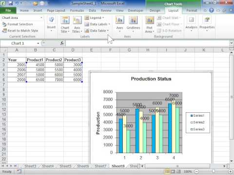
support.microsoft.com › en-us › officeEdit titles or data labels in a chart - support.microsoft.com You can also place data labels in a standard position relative to their data markers. Depending on the chart type, you can choose from a variety of positioning options. On a chart, do one of the following: To reposition all data labels for an entire data series, click a data label once to select the data series.
Format Number Options for Chart Data Labels in Excel 2011 for Mac
› excel_barcode › data_encodingFree Download Excel 2016/2013 QR Code Generator. No barcode ... Create EAN-128 in Excel 2016/2013/2010/2007. Not barcode EAN-128/GS1-128 font, excel macro. Full demo source code free download. Excel 2016/2013 Data Matrix generator add-in. Full demo source code free download. Not barcode Data Matrix font, excel formula. Not barcode font. Generate UPC-A in excel spreadsheet using barcode Excel add-in. No need ...

Excel 2013 Tutorial Formatting Data Labels Microsoft Training Lesson 28.6 - YouTube
Data classification & sensitivity label taxonomy - Microsoft Service ... Data classification levels by themselves are simply labels (or tags) that indicate the value or sensitivity of the content. To protect that content, data classification frameworks define the controls that should be in place for each of your data classification levels. These controls may include requirements related to: Storage type and location

Excel Treemap - Beat Excel!
Use defined names to automatically update a chart range - Office Select cells A1:B4. On the Insert tab, click a chart, and then click a chart type. Click the Design tab, click the Select Data in the Data group. Under Legend Entries (Series), click Edit. In the Series values box, type =Sheet1!Sales, and then click OK. Under Horizontal (Category) Axis Labels, click Edit.

MS Excel 2010 / How to display data labels on the chart - YouTube
How To Analyze Data In Excel: Simple Tips And Techniques - Digital Vidya Row Labels go across the left-hand side of your table [for example Date, Month, Company Name (same as with column labels, it depends on how you would prefer to look at the data, vertically or horizontally)] ... When you select data in Excel 2013 or later, you will see the Quick Analysis button Quick Analysis Excel Button in the bottom-right ...

How to format data labels in excel charts and data elements - YouTube
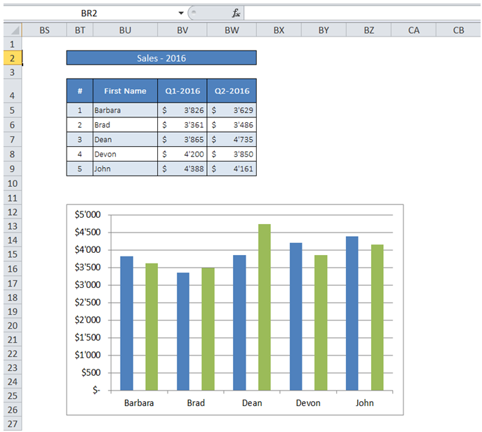
› charts › dynamic-chart-dataCreate Dynamic Chart Data Labels with Slicers - Excel Campus Feb 10, 2016 · Typically a chart will display data labels based on the underlying source data for the chart. In Excel 2013 a new feature called “Value from Cells” was introduced. This feature allows us to specify the a range that we want to use for the labels. Since our data labels will change between a currency ($) and percentage (%) formats, we need a ...

Chapter 3 Excel 2007/2010 Charts
How to Import Data From a PDF to Microsoft Excel - How-To Geek To get started, select the sheet you want to work with in Excel and go to the Data tab. Click the Get Data drop-down arrow on the left side of the ribbon. Move your cursor to From File and pick "From PDF.". Locate your file in the browse window, select it, and click "Import.". Next, you'll see the Navigator pane.
Excel 2010 Remove Data Labels from a Chart - YouTube
How to mail merge from Excel to Word step-by-step - Ablebits On the Mailings tab, in the Start Mail Merge group, click Start Mail Merge and pick the mail merge type - letters, email messages, labels, envelopes or documents. We are choosing Letters. Select the recipients. On the Mailings tab, in the Start Mail Merge group, click Select Recipients > Use Existing List.

Gantt chart with progress - Microsoft Excel 365
Pulling Data Into Excel Power Query - KoBoToolbox Under the Data heading, click on /api/v1/data. Click on GET and select xls. This action will download a text file to your computer called data which can be opened/viewed a text editor. Next, locate your project's data structure inside the data file you downloaded. It will be in the following format: id, id_string, title , description, url.
How to Print Only a Selected Area of An Excel Spreadsheet
How to Make an Excel Box Plot Chart - Contextures Excel Tips Add a blank row in the box plot's data range. Type the label, "Average" in the first column In the remaining columns, enter an AVERAGE formula, to calculate the average for the data ranges. Copy the cells with the Average label, and the formulas Click on the chart, and on the Ribbon's Home tab, click the arrow on the Paste button

Excel 3-D Pie Charts
5 New Charts to Visually Display Data in Excel 2019 - dummies Place text labels describing the data sets above the data. Select the data sets and their column labels. Click Insert → Insert Statistic Chart → Box and Whisker. Format the chart as desired. Box and whisker charts are visually similar to stock price charts, which Excel can also create, but the meaning is very different.

How to Add Data Labels in Excel - Excelchat | Excelchat
How to add text or specific character to Excel cells - Ablebits To add certain text or character to the beginning of a cell, here's what you need to do: In the cell where you want to output the result, type the equals sign (=). Type the desired text inside the quotation marks. Type an ampersand symbol (&). Select the cell to which the text shall be added, and press Enter.

Excel pivot filter – How to filter data in a pivot table
Guide: How to Name Column in Excel - Indeed Career Guide The process of naming columns in Excel entails the steps described below: 1. Change the default column names Locate and open Microsoft Excel on your computer. Removing the actual header's name involves changing the first row of the column you intend to rename. Click inside the first row of the worksheet and insert a new row above the first one.

Enable or Disable Excel Data Labels at the click of a button - How To - PakAccountants.com
Change the Font Size, Color, and Style of an Excel Form Control Label So to change the Label's formatting — even when it's linked to the same cell — you'll need to click the label, click the formula bar, and retype the cell link. Admittedly, everyone else might have already figured this one out. However, I'm still very excited.
Post a Comment for "44 data labels excel 2013"